It didn’t take me long to find the calculus in AP Stats. As someone who never took statistics as an undergraduate (wasn’t required for a math major at my college in the 1980s) and took contextual statistics in graduate school in the 90s (looking at huge data sets with educational research questions in mind), I never had a teacher connect calculus to statistics for me. Until now. Now I am the teacher and the student and my brain started popping with calculus connections this past week in AP Stats.

Before we get to what I connected, two other people made important connections this week because this is what learning is all about — not merely learning the stuff, but connecting the stuff you’re learning to the stuff you already know.

One of the sophomores in our high school noticed a sports car with a Mississippi license plate that said BEOWULF on the Oxford Square. His mom (who is a math teacher in our department) mentioned it to me. She was so delighted that her son recognized something from school out in the world. She was intrigued about the story and got to hear a 10-minute Beowulf synopsis from her son. She was also curious about why someone would have that as their license plate. I could answer that one! That’s Dr. Hall, a University of Mississippi professor (retired but still writing) and Old English scholar. If you’re going to get a vanity plate, it should reflect your passion. Come to my classroom and you’ll see Mark Kiraly’s DX/DT car tag.

Another connection was one our youngest son made. Mom! When did we get this South Park ornament? Now, this Cartman ornament has been on our tree for years. But our son did not notice it because though South Park is a cartoon, the show isn’t exactly appropriate for a younger crowd. As a mom, I wish my child were noticing Beowulf and not South Park, but there’s always next year when he’s a sophomore in Honors English.

Thus, it makes perfect sense that while others notice Beowulf and Cartman, I notice Calculus.

We don’t see things as they are, we see things as we are. — Anaïs Nin

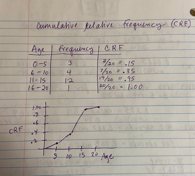
The first AH HA moment was when I plotted a cumulative relative frequency graph as part of my homework assignment. I had never seen a graph like that in statistics before. But I had seen plenty of those in calculus — I was sketching the antiderivative by way of an accumulation function. What was this graph telling me? For one thing, percentiles were easy to determine and also where the slope is steep you’ll have your greatest frequency! If we sketch the derivative of the cumulative relative frequency graph, TA DA, the distribution graph!

Then, as I was preparing to teach about calculating, interpreting and using z-scores, I thought to myself, Wait a minute. Forget this Table A nonsense to match the z-score to the percentile. Surely there is an equation for the standard normal curve. If I knew the equation, I could just integrate with the z-score(s) as the limits of integration and get my result faster. I imagined the derivative of the cumulative frequency graph to be f(x) = k/(1+x^2) and after fooling with that for a while without landing on some key results, I reached out to my math family. They pointed my in the direction of a German mathematician.

Come to find out, Gauss figured all this out (among lots of other things such as how to calculate Easter’s date) way before my time, and even way before statistics was even a thing. You can see the accumulation function and the standard normal curve on this Deutsche Mark I found at leftovercurrency.com.

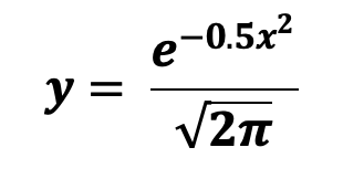
It’s a little bit hard to see on the paper money, but the equation printed on it includes the mean (mu) and the standard deviation (sigma). If you have already converted your value(s) to a standard score (z-score), the mean and standard deviation are not needed.

Thus the equation becomes

The graph of the equation looks like this:

And to find the percent of values that fall within 1 standard deviation of the mean, find the area under the curve from -1 to 1. You’ll need calculus! You’ll also need a calculator or perhaps some advanced techniques, but I am not sure if this is doable even with advanced techniques.

Woah. There’s 2/3 of the empirical rule… 68 – 95 – 99.7. KA BOOM.

That’s enough for one blog post — I think I lost a lot of you after the South Park connection and thank for reading until the end anyway. As I promised last time, stay tuned for another AP Stats update as I continue my journey into uncharted territory.